.jpeg)
Predicting Steel Product Order Quantity Using LSTM (Long Short-Term Memory) Machine Learning Technique: Demand Forecasting Using Multivariate Time Series Data
LSTM(Long Short-Term Memory) 머신러닝 기법을 이용한 철강 제품 주문량 예측: 다변량 시계열 데이터를 활용한 수요 예측
1 한국대학교
1 Hankuk University
DOI: https://doi.org/10.17287/kbr.2025.29.4.113
초록
본 연구는 다변량 시계열 예측 모델인 LSTM(Long Short-Term Memory) 신경망을 활용하여 철강 산업의 수요 예측 문제에 대한 새로운 접근 방식을 제시한다. 철강 산업은 생산 공정의 복잡성, 리드 타임의 증가, 시장의 불확실성으로 인해 수요 예측에 높은 가치를 두고 있다. 제안된 방법론은 머신러닝 기법을 사용하여 다변량 LSTM 모델을 개발하고 다양한 지표를 사용하여 성능을 평가한다. 또한 철강 산업의 고유한 특성에 맞추기 위해 산업 전문가의 통찰력을 바탕으로 변수 선택을 수행하였다. 결론적으로 본 연구에서 개발된 LSTM 모델은 기존의 수요 예측 방법보다 우수한 성능을 보였다. 특히 복잡한 시장 트렌드와 철강 산업의 특성을 정확하게 반영하여 보다 정밀한 수요 예측을 가능하게 한다. 본 연구는 철강 산업의 수요 예측 문제에 대한 새로운 솔루션을 제시하며, 이는 생산 계획 및 재고 관리의 효율성을 향상시킬 것으로 기대된다.
Abstract
This study presents a novel approach to the demand forecasting problem in the steel industry, utilizing a multivariate time series forecasting model, specifically the Long Short-Term Memory (LSTM) neural network. The steel industry places a high value on demand forecasting due to the complexity of its production processes, increasing lead times, and market uncertainty. The proposed methodology uses machine learning techniques to develop a multivariate LSTM model and evaluates its performance using various indicators. Additionally, to align with the unique characteristics of the steel industry, we performed feature selection based on the insights of industry experts. In conclusion, the LSTM model developed in this study outperforms existing demand forecasting methods. Specifically, it accurately reflects complex market trends and the characteristics of the steel industry, enabling more accurate demand forecasting. This study presents a novel solution to the demand forecasting problem in the steel industry, which is expected to enhance the efficiency of production planning and inventory management.
Ⅰ. Introduction
The steel industry, which forms the backbone of manufacturing worldwide, is a vital sector that supplies raw materials to various industrial fields, including construction, automobiles, shipbuilding, and machinery. Steel products undergo a complex manufacturing process comprising more than five stages, from iron ore smelting to plating, depending on the product's composition and characteristics. In particular, the steel industry is not a supply chain that responds to sudden orders because it necessitates planned production due to its minimum production volume, large-scale facilities, and diverse product line. Additionally, because the lead time is at least two months, if the order is not placed promptly, it may take more than three to four months after the product is ordered.
This study targeted small and medium-sized companies that manufacture corrugated steel pipes. A corrugated steel pipe is formed by assembling hot-rolled steel into a corrugated shape and then coating it as needed. It has a relatively high strength, durability, and economic efficiency. Due to these characteristics, corrugated steel pipes are utilized in the construction of roads, railways, and airports, as well as in various civil engineering projects, including bridges, tunnels, drainage ditches, and industrial piping systems. It is an industry that attracts attention as its use increases in infrastructure construction in each country. Due to the diverse fields of use for corrugated steel pipes, manufacturers must respond promptly to fluctuations in demand across various industries. Delivery is considered as important as unit price and quality in winning contracts.
Numerous factors, including economic volatility, policy changes, and fluctuations in raw material prices, influence the steel industry. It has the characteristic that causes significant fluctuations in demand, according to these changes. In particular, with the increasing uncertainty in the global economy, demand forecasting for steel products is becoming more important. Moreover, the production process of steel products is complex and resource-consuming, making it difficult to control production quickly. Therefore, it is essential to accurately predict the demand for steel products and establish production plans in advance. This study aims to predict the optimal order quantity of hot-rolled coil used in the manufacture of corrugated steel pipe. Hot-rolled coil is a crucial steel form and a vital raw material for manufacturing corrugated steel pipes. Corrugated steel pipe manufacturers can create effective production plans by forecasting demand for hot-rolled coils, efficiently purchasing raw materials, and effectively managing inventory.
Make-to-order (MTO) is a manufacturing method that produces products as soon as an order is received. It is mainly used in the corrugated steel pipe industry. (Schroeder, 2013) This method's biggest advantage is minimizing product inventory and increasing production efficiency. However, this approach has certain challenges, including ordering raw materials and managing inventory. Corrugated steel pipe manufacturers must establish effective strategies to maintain a reasonable level of raw material inventory while ensuring a smooth production process for orders. It is called safety stock and can be said to complement the weaknesses of the order production method. As one of these strategies, accurately predicting the order level of hot-rolled steel sheets is crucial to purchasing raw materials and managing inventory effectively.
The company subject to this study determines the timing of ordering below the average inventory level based on average consumption, the highest inventory volume, and the safety stock volume, and calculates demand linearly. However, demand behavior is non-linear, and the only way to deal with the rapidly rising order volume in the early stages of a project is to delay delivery.
It takes three months from steel manufacturing through the toll processing process to stocking at the factory. A high safety stock is needed to respond to unexpected demand. However, inventory management fails due to the high price per unit and high inventory costs, which are characteristics of steel products. There is a risk that small and medium-sized businesses may not be able to cover costs and go bankrupt. On the other hand, there are quality disadvantages, such as surface oxidation or deterioration that can occur during long-term storage. Therefore, from a quality control perspective, only an appropriate level of raw material inventory must be maintained.
In addition, this paper helps to understand research trends in raw material purchase timing decisions that predict non-linear demand through research on multivariate time series forecasting using Long Short-Term Memory (LSTM) models. It suggests future research based on these findings. This paper provides a methodology that can be applied to demand forecasting in the steel industry and other industrial fields. Based on this, it aims to contribute to solving general problems in demand forecasting.
Ⅱ. Theoretical Background
2.1 Related Works
(Danilczuk et al., 2022; Towill & Christopher, 2010) presented the need for demand forecasting using the order production method. (Kuthambalayan & Vera, 2020) proposed a hybrid greedy and non-linear branch production strategy and a mixed MTS-MTO production system using semi-finished products, pursuing a flexible yet efficient production method. Martin reported that some companies have attempted to improve their supply chain strategies by incorporating demand forecasting into traditional make-to-order methods. (Danilczuk et al., 2022) Through this, we increased the efficiency of the supply chain and minimized risks in inventory management and raw material purchases.
(Martinez-de-Albeniz & Simchi-Levi, 2005) developed a demand forecasting model using the portfolio approach of ordering contracts using the order production method. (Das & Kuthambalayan, 2022) reported a marketing model related to lead time-dependent demand-supply matching in the MTO method. A solution to the unconstrained stochastic non-linear problem was presented by deriving a mathematical model that finds the trade-off between safety inventory cost, lead-time guarantee, product price, and operating profit.
Time series demand forecasting has been studied in various fields, and machine learningbased forecasting, particularly in the era of big data, is gaining recognition as a growingly important area. (Seyedan & Mafakheri, 2020) Among various demand forecasting techniques, neural network-based demand forecasting was adopted the most, followed by general regression, time series analysis (ARIMA), and support vector machine (SVM) decision tree methods.
In machine learning-based forecasting models, nonlinear demand forecasting has improved, but the accuracy of order forecasting remains a significant issue. (Seyedan & Mafakheri, 2020; Rivera-Castro et al., 2019) Various methodologies have been proposed, such as the random forest, gray model, support vector machine, and neural network. However, among them, the methodology of using LSTM (long short-term memory) has recently shown notable results. (Dou et al., 2021) used LSTM to predict demand for regional manufacturing industries at the highest level compared to other machine learning techniques.
(Moalemet et al., 2022) applied LSTM to predict electricity demand at a steel mill and showed higher prediction accuracy than existing methodologies. This paper demonstrated that LSTM effectively learns complex patterns over time and can accurately predict future demand based on these patterns. Furthermore, Kim and Jeong (2019) developed a demand forecasting algorithm within a smart factory using an advanced hybrid model that improves forecasting performance by dividing existing demand forecasting techniques into short-term, mid-term, and long-term categories. In the short term, predictions were made using a combination of exponential smoothing, LSTM in the medium term, and ARIMA in the long term, and it was claimed that these methods generally provided more accurate predictions.
Meanwhile, a study on demand forecasting in cases where demand fluctuations are very large (Kim & Jeong, 2019) predicted demand for smart factories using the ARIMA method and LSTM, and employed regularization techniques to identify key factors that affect demand forecasting for each CPU and server semiconductor. The demand for the semiconductor cycle was predicted by deriving factors and clustering demand patterns.
2.2 Production Planning Method
The production planning method is determined based on customer requirements and the company's production and inventory management strategy. Four major methods are widely used. The representative production planning methods are ‘Make to Stock (MTS)’ and ‘Make to Order (MTO)’. The other three are ‘Assemble to Order (ATO)’, ‘Make to Order (MTO)’, and ‘Engineer to Order (ETO)’. (Schroeder, 2013)
Manufacturing to stock (MTS) involves producing products in advance, storing them in inventory, and supplying them to customers upon request. This method minimizes the time interval between production and supply and is suitable when market demand is predictable and volatility is relatively low.
Assemble-to-order (ATO) is a method of assembling products according to the customer's order after it is received. Some products are produced in advance and stored in inventory, but the final product is assembled after the order is placed. It is an intermediate form between MTS and MTO. It holds inventory in the form of intermediate products or major parts and then assembles them into finished products upon customer order. Manufacturing to Order (MTO) begins product production upon receipt of a customer's order. This method can significantly reduce product inventory costs and provide customized products. However, since product production begins after the order is placed, the supply time may be longer than MTS or ATO. Design-to-order (DTO) is a process where a product is designed according to customer requirements and then produced according to the design. This approach enables highly customized product offerings that cater to the complex or unique needs of individual customers.
2.3 Traditional Demand Forecasting Method
Demand forecasting is crucial for managing a company's production plan, inventory, and dictions are generated using a range of methodologies, each with its strengths and weaknesses. (Wisner, 2016) Among the existing demand forecasting methodologies, the most widely used is time series analysis, which includes moving averages and exponential smoothing methods, and predicts future sales volumes based on past sales data. Many companies have preferred this statistical method due to its simplicity and ease of interpretation. However, they assume that past data patterns will continue, which is not always the case in real market conditions. Additionally, statistical methods have limitations because they struggle to effectively handle complex, nonlinear patterns or multivariate time series data. The moving average method predicts future values by calculating the average of data over a specific period for time series data analysis. This method is effective for data where trends or seasonality are not readily apparent, and is also advantageous in reducing noise in time series data. The exponential smoothing method is a weighted moving average approach that more rationally addresses the weaknesses of the moving average method, specifically the irrationality of weight selection criteria and the determination of the target period N. Meanwhile, the ARIMA (Auto Regressive Integrated Moving Average) model is one of the core methodologies for analyzing time series data and is particularly effective in predicting linear patterns based on temporal changes in the data. (Kang, 1978) In contrast, machine learning-based demand forecasting methods excel at handling nonlinear patterns and multivariate data. It can provide more powerful solutions to real-world problems where multiple factors affect demand. However, machine learning methodologies have the disadvantage that model interpretation is more challenging than statistical methodologies, and problems such as overfitting may arise.
In this study, we propose a demand forecasting methodology that utilizes the Long Short-Term Memory (LSTM) model. LSTM performs exceptionally well in processing data with long-term dependencies, which is particularly useful for complex time series data, such as demand forecasting for steel products.
Additionally, LSTM has an excellent ability to process multivariate time series data. It is a crucial factor in predicting the demand for steel products, as various factors, including market conditions, economic environment, and shifts in customer demand, influence it. Using LSTM, demand can be predicted by considering these various factors simultaneously, resulting in more accurate forecast results. Using these advantages of LSTM, a demand prediction model for steel products was developed. This model overcomes limitations found in existing methodologies, allowing more accurate and reliable demand forecasting results to be derived.
2.4 LSTM Time Series Forecasting Method
Long Short-Term Memory (LSTM) is a type of Recurrent Neural Network (RNN) that excels at processing time series data. LSTM enhances the structure of the basic RNN, enabling it to learn long-term patterns in time series data. This property is particularly useful in problems such as demand forecasting, where patterns over time are important.
Additionally, LSTM can process multivariate time series data. Predictions can be made by considering multiple time series data simultaneously. For example, various factors such as product type, price, supplier's production capacity, and competitor situation can be considered when forecasting demand for steel products.
However, there are several caveats when using LSTM. Because LSTM has many parameters, overfitting problems may occur when the training data is insufficient. Additionally, since learning an LSTM model is time-consuming and computationally intensive, an appropriate model structure and learning strategy must be selected, considering these factors. As such, LSTM can effectively process time series data and is well-suited for applications such as demand forecasting for steel products. LSTM enables the learning of complex patterns in time series data and the prediction of future demand by considering multiple factors simultaneously. It enables limitations found in existing forecasting methodologies to be overcome, thereby improving demand forecasting accuracy.
In this study, a demand forecasting model for steel products was developed using Long Short-Term Memory (LSTM) networks. It presented a new approach to the demand forecasting problem in the steel industry, and the advantages of LSTM could be considered an alternative to the existing safety stock.
Ⅲ. Research Methodology
3.1 Data Collection and Preprocessing
To learn LSTM demand forecasting, order quantity data for steel products from small and medium-sized companies that produce corrugated steel pipes was collected from their ERP systems. The main characteristics are that large-scale projects occur, orders exceeding 1,000 tons are processed per month, and the cycle is not constant. Also, there is a characteristic that the low-order volume persists for approximately three months after a large order is placed.
Additionally, relevant statistical data and reports were collected to reflect external factors, including economic indicators and trends in the steel market.1 The data collected this way was used to understand demand patterns for steel products and predict future demand.
The preprocessed data was divided into training data and test data. Of the training data, 70% was used for learning and 30% for validation. Data from the last 24 months was used as test data to evaluate prediction performance. A method is implemented where the model learns from past patterns and predicts future demand based on these. The training data constructed this way was used to train the LSTM model. Each input sequence includes features such as order quantity for the past $n$ months, construction material index, construction economy statistics, industrial production index, other construction raw materials, and hot-rolled futures index.
3.2 Multivariate Variable Selection and Model Structure
This study selected various variables to predict demand for steel products. The selected variables mostly included orders for steel products and economic indicators related to the steel market.
Meanwhile, the LSTM model developed in this study comprises an input layer, a hidden LSTM layer, and an output layer. The input layer accepts variables such as demand for steel products, construction economy statistics, the construction material index, the industrial production index, other construction raw materials, and the futures index. It passes this information to the hidden Long Short-Term Memory (LSTM) layer. The hidden LSTM layer updates its internal state based on this input information, which is used to remember past events and predict future outcomes. Finally, the output layer predicts the order quantity of steel products for the next three months based on the internal state of the LSTM layer.
The model's learning was conducted to minimize the difference between the predicted and actual output for a given input sequence. For this purpose, this study used the Mean Squared Error (MSE) loss function and the Adam optimization algorithm. The Early Stopping technique, included in Keras, was also applied during the learning process to prevent overfitting.
3.3 Learning and Evaluation Methods
In this study, we adopted a clear and systematic approach to learning and evaluating multivariate long short-term memory (LSTM) models. This section provides a detailed description of these methods, discussing the primary techniques and metrics employed for training and evaluating LSTM models.
The multivariate LSTM model is learned through backpropagation, which occurs in temporal order. It enables the model to learn the patterns in time series data effectively. Adam (Adaptive Moment Estimation) was used as an optimization algorithm to learn the LSTM model. Adam adaptively adjusts the learning rate, showing effective performance in complex models such as LSTM.
This study divided the entire dataset into learning, validation, and testing datasets to determine the model's predictive performance. It is done to prevent the model from overfitting and obtain results that more accurately reflect its actual performance. Additionally, this study employed a learning curve to monitor changes in model performance throughout the training process. The learning curve visualizes the training loss and validation loss by epoch, enabling them to monitor the model's learning status in real-time. Through this process, problems such as overfitting and the learning rate were identified and promptly adjusted.
The performance of an LSTM model is highly dependent on the selected hyperparameters. Therefore, finding suitable hyperparameters is crucial for optimizing model performance. This study employed a grid search to identify the hyperparameter combination that yielded the best performance. Grid search is a method of exploring all possible hyperparameter combinations and evaluating the performance of each combination to find the optimal combination.
Through this method, this study systematically conducted the learning and evaluation of a multivariate LSTM model for predicting demand for steel products. It ensures effective learning and accurate performance evaluation of the LSTM model, which is crucial for enhancing prediction performance in real-world situations. This approach can be applied to demand forecasting in the steel and various other industries, leading to more effective inventory management and production planning. The primary indicators used to evaluate the model's performance were the mean absolute error (MAE), the mean absolute percentage error (MAPE), and the root mean squared error (RMSE).
Ⅳ. Research Results
4.1 Linear Demand Forecasting Techniques (Moving Average, Exponential Smoothing, ARIMA)
The conventional moving average method was employed to compare LSTM performance and serve as a comparison group. The moving average method is a simple yet effective way to reduce noise in time series data and clearly express the underlying structure of the data. In this study, we employed the moving average method to predict demand over the last 24 months and compared the results with the actual values.
According to the experimental settings, the window size of the moving average method was set to 6. Each forecast reflects the average demand over the previous six months. As shown in Figure 1, the Root Mean Square Error (RMSE) of the prediction performed under this setting was measured to be 143 tons. RMSE is the square root of the mean square error between predicted and actual values. A lower value means better prediction performance.
The moving average method had the advantage of being simple to calculate and having a fast calculation speed; however, forecasting using this method had several limitations. Because the moving average method relies on linear patterns in data, predicting periods of high volatility, such as rapid increases in order volume, has been difficult. Additionally, because the moving average method makes predictions using only past average values, it does not accurately reflect complex patterns in time series data, such as trends or seasonality. These results suggest that the moving average method can only match the trend at a basic level. It is an important point to consider in the follow-up work of this study, suggesting the need to introduce a more complex time series prediction model.
The exponential smoothing method in this study was performed by setting the smoothing coefficient to 0.2. It was implemented using the Exponential Smoothing class of ‘statsmodels’, and this class performs predictions by assigning different weights to past data at each point in time. Using the exponential smoothing method established in this matter, demand for the last 24 months was predicted and compared with the actual value. As a result, the RMSE of the prediction using this method was measured to be 148 tons. It represents 444 tons, the tolerance value measured at the 3-sigma level of prediction performance, indicating that a difference of up to 20 coils or more can occur. (Figure 2)
While the exponential smoothing method demonstrated comparable performance to the traditional safety stock setting and linear operation, its ability to predict non-linear patterns was limited. Due to its assumption of a linear pattern, which challenges forecasting scenarios such as a sudden surge in order volume. As a result, the method was constrained to tracking trends, a significant limitation identified in this study.
The ARIMA demand forecasting technique is called the Python Stats model library and utilizes the ARIMA method. In the ARIMA model, p, d, and q each have the following meanings. The p-value corresponds to the order of the autoregressive (AR) part, which describes the degree to which past values influence current values. The d value refers to the order of difference required to convert the original time series data into data with stationarity. The $q$ value is the order of the moving average (MA) portion. It explains how past forecast errors affect current values. These three parameters must all be non-negative integers; the larger the value, the more information the model must consider, thereby increasing computational complexity. Selecting suitable values for these parameters substantially impacts the model's performance. In this study, the $p$-value was changed from 1 to 12, the $d$-value was changed from 0 to 5, and the $q$-value was changed from 0 to 5 (i.e., 12, 1). When set to 2, irregular behavior was shown to be predicted to some extent. The RMSE of the ARIMA method was at the 129-ton level, showing the best performance among linear prediction techniques.
4.2 Univariate LSTM
An attempt was made to improve the accuracy of steel demand forecasting by applying the LSTM model. LSTM is widely recognized as a structure that can effectively identify long-term patterns in time series data. This attempt aims to overcome the limitations of existing linear methods, specifically their inability to predict when order quantities fluctuate rapidly. The experimental setup focuses on demand forecasting for steel products. The basic settings for various elements for this are as follows.
Data Set: The data used in the univariate LSTM model experiment are the order volumes of steel products over the past 12 years. ERP provided this data to a steel manufacturer, allowing it to reflect the complexity and diversity of actual industrial sites. There were 158 months of data, of which 94 months (approximately 60%) were used for learning, 40 months (approximately 25%) were used for validation, and the remaining 24 months (approximately 15%) were used as test data.
Model setup: The LSTM model consisted of two LSTM layers and one fully connected (Dense) layer. The LSTM layer is responsible for remembering information for a long period and predicting the future based on it. The Dense layer receives the output from the LSTM layer and generates the final predicted value. The number of neurons in the LSTM layer was set to 50 and 100, respectively, and the number of neurons in the Dense layer was set to 1. Based on data from the past six months, the model set up in this way predicts the order quantity of steel products for the next three months.
Training setup: The Adam optimization algorithm and Mean Squared Error (MSE) loss function were used to train the LSTM model. The Adam optimization algorithm dynamically adjusts the learning rate for each parameter, and the MSE loss function minimizes the squared difference between the actual and predicted values. Additionally, Early Stopping and Dropout techniques were applied to prevent overfitting. Early Stopping is a technique that terminates learning early if performance on the validation dataset does not improve for a certain period. Dropout is a technique that controls the complexity of the model by randomly deactivating some neurons during the learning process.
Accordingly, this study implemented a univariate LSTM model. Through this, we predicted steel demand for the last 24 months and measured the prediction performance by comparing it with the actual value. As shown in Figure 4, the Root Mean Square Error (RMSE) of the LSTM prediction was measured to be 158 tons. It indicates that a difference of up to 25 coils or more occurred when compared to the tolerance value of 474 tons, allowing for a prediction error at the three-sigma (99.7%) level.
However, these results suggest that predictions through the LSTM model have not reached a practical level. In the corrugated steel pipe manufacturing industry, which accounts for a significant portion of fixed costs, this level of forecast error results in substantial increases in inventory costs, leading to substantial economic losses. It can be especially problematic in MTO systems. In the MTO method, production begins after an order is received, so it is crucial to accurately predict the order's timing. However, the univariate LSTM model in this study had difficulty predicting these order timings. Based on these results, this study will consider ways to improve the performance of the LSTM model in the next section. To this end, it plans to optimize the learning method of the LSTM model through hyperparameter tuning.
4.3 Univariate LSTM Hyperparameter Adjustment
In this study, we considered hyperparameter tuning to improve the performance of univariate LSTM models. Among various hyperparameters, we sought to improve the model's prediction performance by tuning the lookback value, epoch value, batch size value, number of LSTM neurons (units), number of neural network layers, and learning rate.
In conclusion, changes in the lookback value had the greatest impact on prediction performance among all hyperparameters. It confirmed that utilizing past information at appropriate time intervals plays a critical role in improving the performance of the LSTM model.
In this study, 100,800 calculations were performed considering the combination of hyperparameters considered above. The final result obtained through these extensive calculations showed an RMSE of 102 tons, which is superior to previous prediction methods. However, this figure remains outside our acceptable range.
The primary challenge in forecasting using only univariate LSTM was that it required time to accurately predict the timing of a rapid increase in order volume. Although LSTM effectively predicts the future by learning from past time series data patterns, it can easily miss important information, such as the timing of orders. This study's prediction was also performed using only a single variable, past order quantity. Although this method fully understands the patterns of time series data, it cannot account for other factors that may explain the increase in order quantity. For example, various external factors such as economic conditions at a specific time, changes in customer behavior, and market volatility significantly impact order quantity. Still, because these factors were not included in the univariate forecasting model, forecasting performance was limited.
As a result, the performance of the prediction model using LSTM improved. However, eliminating or reducing the prediction error to an acceptable range still needs improvement. Future research should aim to develop more accurate methods for predicting rapid increases in order volume using multivariate analysis.
4.4 Comparison of Multivariate LSTM and Prediction Performance
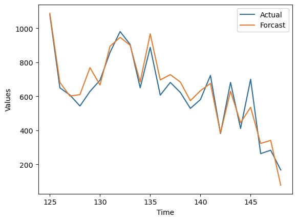
Figure 5 presents the results of the Train Test values for actual and predicted demand for raw steel materials after adding variables to the multivariate LSTM model and tuning a series of hyperparameters, following a similar process to the one described in the previous section.
First, the demand forecast should be based on the construction and civil engineering industry. The possibility of using it for orders increases significantly, reflecting the trend. While the existing linear demand forecasting technique, or univariate LSTM method, relies on a single indicator, the multivariate LSTM model enables more accurate demand forecasting by utilizing multiple indicators, such as those related to the construction and civil engineering economy.
One powerful advantage of these multivariate LSTM models is their ability to predict rapid increases in demand. Rapid fluctuations in demand significantly impact a company's production and orders, making it crucial to predict them accurately. The multivariate LSTM model can predict this rapidly changing demand by considering various indicators together, which allows companies to establish production plans more efficiently.
Figure 6 displays the order volume and forecast for the past 24 months. The RMSE indicates an error of 53 tons in the monthly forecast. It can be calculated as 159 tons based on $3\sigma$ (99.7%), which can be understood as an error that occurs at the level of about seven coils. This level of error is acceptable in actual practice, considering storage costs. This figure was attainable because the rapid demand forecast was partially predicted and is presumed to have been derived from various variables and appropriate lookback values. Additionally, such accurate predictions greatly help shorten delivery times, ultimately leading to favorable results in winning orders. Therefore, these prediction models can be very useful in management activities.
In this manner, the multivariate LSTM model outperforms existing demand forecasting techniques. However, applying advanced optimization techniques or adding more effective time series features that predict order timing can improve performance. Research and further attempts on this need to continue.
The multivariate LSTM model outperforms existing demand forecasting techniques, particularly in predicting rapid demand changes and capturing trends. It enables companies to establish more efficient production and order plans and obtain valuable data for management activities. Further developing this model is an important task at present.
The LSTM model's performance was compared with existing time series forecasting methodologies. The performance comparison was based on the root mean square error (RMSE), and the results obtained are presented in Table 1
Table 1 Performance comparison of demand forecasting techniques
| Model | MAE | MAPE | RMSE |
|---|---|---|---|
| Moving Average | - | - | 143 |
| Exponential Smoothing | - | - | 148 |
| ARIMA | - | - | 129 |
| Univariate LSTM | - | - | 158 |
| Univariate LSTM (Tuned) | - | - | 102 |
| Multivariate LSTM | Low | Low | 53 |
These results show that the multivariate LSTM performs best. The Multivariate LSTM, which yielded the lowest values in all indicators of MAE, MAPE, and RMSE, was the technique that produced the lowest prediction error. It is because a multivariate LSTM performs predictions by considering multiple variables simultaneously. Since world demand results from the interaction of various complex factors, LSTM, which can handle such multivariate variables, can well reflect this situation. This improvement in prediction performance is compared to other methods that use a single variable.
Overall, these performance comparison results clearly show that in actual demand forecasting, various factors interact in a complex manner to determine demand. Therefore, multivariate LSTM, which can account for all these factors, provides the most accurate prediction. Of course, even when using a multivariate LSTM, the importance and interaction of each variable must be properly considered, and a sufficient amount of data and an appropriate learning algorithm are also required. However, upon careful consideration, multivariate LSTM can be a highly effective tool for demand forecasting.
4.5 Variable Importance Analysis
The multivariate LSTM model employed in this study enhanced predictive performance by utilizing various economic indicators and historical order data as input variables. However, the model's structure makes it difficult to explain “why a particular prediction was made directly.” To address this, an interpretability technique (Explainable AI) was applied after model training. For the 13 input variables used in this study, variable importance was analyzed using SHAP (SHapley Additive ex Planations) values and the Permutation Importance technique.
The SHAP (SHapley Additive ex Planations) value is an interpretation technique based on cooperative game theory that quantitatively assesses the contribution of each input variable to model predictions. A higher absolute value of a SHAP value generally indicates a greater influence of the variable on the model output. For example, a SHAP value of 0.05 or higher indicates a significant contribution to the prediction, while a value closer to 0 indicates a minimal influence.
Permutation Importance is a technique that measures the performance degradation (e.g., increased Root Mean Square Error) that occurs when the values of a specific variable are randomly shuffled, based on the predicted performance of a trained model. A larger increase in RMSE indicates that the variable plays a significant role in model performance. For example, an RMSE increase of 10 tons or more indicates a significant impact on predictive performance, while an RMSE increase of 2 tons or less indicates a minor impact. Permutation Importance mitigates model opacity (black-box) issues and has the advantage of being applicable regardless of model structure.
It was executed to increase model interpretability and identify the factors that have the most significant impact on prediction results. The analysis results identified rebar domestic supply and rebar production as the most important variables. The domestic supply of rebar had a SHAP value of 0.090 and a 9.2-ton increase in RMSE in the permutation importance analysis. It suggests that these variables make a significant contribution to model prediction accuracy. Following this, civil engineering (public) (SHAP = 0.072, RMSE = 7.1 tons) and galvanized steel production (Galvanized Steel Prod., SHAP = 0.062, RMSE = 7.0 tons) were identified as being of high importance. Conversely, primary metal products (PPI) showed the lowest importance, with a SHAP value of 0.027 and an RMSE of 2.7 tons, indicating a limited relative influence. (Table 2
Table 2 Variable Importance Analysis Results
| Variable | SHAP Value | RMSE Increase (tons) |
|---|---|---|
| Rebar Domestic Supply | 0.090 | 9.2 |
| Rebar Production | - | - |
| Civil Engineering (Public) | 0.072 | 7.1 |
| Galvanized Steel Prod. | 0.062 | 7.0 |
| Primary Metal Products (PPI) | 0.027 | 2.7 |
These results demonstrate that variables closely related to steel supply and demand (domestic demand, production, and construction performance) play a key role in demand forecasting, and that price indicators alone have limited explanatory power. However, some variables contributed only slightly to improved forecast performance, suggesting the need to reexamine variable selection strategies for future model simplification and performance optimization. Moreover, LSTM models reflect interactions between input variables, making it difficult to isolate the influence of individual variables completely. Therefore, SHAP and Permutation Importance should be used as reference metrics; results may vary depending on the data characteristics and model structure. (Figure 7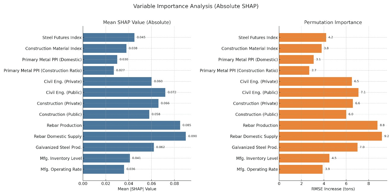
Ⅴ. Concluding Remarks
In this study, we developed a model to predict order quantities in the steel industry using a multivariate Long-Short-Term Memory (LSTM) neural network. This model effectively captures the characteristics of complex time series data and can accommodate a range of external variables. It showed higher performance than existing time series forecasting methodologies in predicting order quantities in the steel industry.
The results of this study show that the LSTM model can effectively solve complex time series prediction problems. The LSTM model enables predictions that consider complex patterns and various external variables through its ability to process data with long-term dependencies and multivariate time series data. Future research can explore various LSTM structures and identify ways to further enhance the performance of the LSTM model by comparing it with other time series prediction models. Additionally, it can improve the model's prediction accuracy by more accurately analyzing the effects of various external variables.
5.1 Future Research Directions
This study confirmed that an LSTM-based multivariate time series model outperforms traditional forecasting methods (moving average, ARIMA). However, further research is necessary to address the complexity of industrial environments and the changing characteristics of data. To further improve forecast accuracy and interpretability, the following extensions are proposed.
-
Introduction of an Attention Mechanism and Reflection of Seasonality: The attention mechanism has the advantage of dynamically learning the importance of specific time points or variables in time-series data, thereby mitigating the long-term dependency problem of LSTMs. Steel demand, in particular, is strongly influenced by the construction cycle and seasonal factors, so simply inputting these patterns as a time series is insufficient. Future research should incorporate seasonality as a categorical variable and pay attention to reflect the interactions between variables and the importance at each time point. It is expected to enable the forecasting model to learn the characteristics of specific periods more precisely (e.g., a decrease in construction demand during the winter season, a surge during the peak season).
-
A Comparative Study of GRU (Gated Recurrent Unit): GRUs have a simpler structure and fewer training parameters compared to LSTMs, offering advantages in computational efficiency and learning speed. In environments with a limited dataset size or real-time predictions, GRUs may be more suitable. Therefore, further research is needed to compare the performance of GRUs and LSTMs based on the same variable set and quantitatively assess factors such as the number of parameters, training time, and the likelihood of overfitting. In particular, given the difficulty of securing all influencing variables in real-world industrial settings, it is necessary to examine whether the simplified GRU structure can contribute to improved prediction stability in practice.
-
Transformer-based Model Exploration and Hyperparameter Optimization: In this study, a grid search was employed to identify the optimal parameters. However, this method suffers from limitations, including a limited search scope and high computational costs. Exploration techniques based on Bayesian Optimization, Hyperband, and AutoML can improve search efficiency and automatically derive optimal performance. In particular, automating optimized parameter settings for various model structures, such as LSTM, GRU, and Transformer, will significantly enhance practicality in industrial applications.
-
Expanding Data Diversity and Reflecting External Factors: The current model is limited to internal order data from ERP and some macroeconomic indicators. However, actual steel demand is influenced by external factors, including project size, regional construction market trends, global raw material prices, competitor trends, and policy changes. Therefore, future research needs to integrate diverse external data and enhance data cleansing and feature engineering techniques. In particular, developing models that integrate unstructured data (e.g., news articles, policy reports) can simultaneously improve forecast accuracy and timeliness.
5.2 Practical Implications and ERP Integration
The LSTM-based demand forecasting model proposed in this study can significantly enhance the efficiency of supply chain management (SCM) decision-making by integrating it with Enterprise Resource Planning (ERP) systems. Specifically, by implementing features that automatically adjust order timing and safety stock levels, it can complement the limitations of existing empirical and fixed decision-making methods.
Current procurement methods are primarily based on historical average consumption and fixed safety stock levels, making it difficult to respond quickly to economic fluctuations or large-scale orders early in a project. It often leads to order delays that exceed the average lead time of two to three months, potentially resulting in delayed delivery and penalties. In contrast, integrating the proposed predictive model with an ERP system enables the prediction of demand in advance and the generation of timely orders. For example, if an LSTM model predicts demand for approximately 1,200 tons of steel over the next three months, the ERP procurement module can automatically generate purchase requisitions based on this forecast. This process accelerates the ordering process compared to conventional methods, minimizing the risk of delivery delays due to inventory shortages. Furthermore, by optimizing safety stock, inventory holding costs can be significantly reduced.
Quantitative simulation analysis results showed that under the existing operating method, average monthly inventory was maintained at 1,000 tons, resulting in storage costs of approximately 30 million won. In contrast, the predictive model-based optimization scenario reduced the average monthly inventory to 850 tons, resulting in monthly storage costs of approximately 25.5 million won, which translates to a savings of approximately 4.5 million won (approximately 15%). By avoiding potential penalties for late delivery (approximately 5 million won per case), the annual savings could exceed tens of millions of won.
ERP-integrated predictive operations system holds significant potential not only in make-to-order (MTO) manufacturing but also in various industries with long lead times and high demand volatility. Additionally, by integrating the model proposed in this study with a manufacturing execution system (MES) or a supply chain management (SCM) platform outside of an ERP, comprehensive optimization encompassing production planning, purchasing, and logistics planning can be achieved. It is expected to lead to strategic outcomes beyond simple cost savings, including enhanced supply chain resilience and improved delivery reliability.
Ⅵ. Conclusion
This study developed and validated a multivariate LSTM (Long Short-Term Memory)-based demand forecasting model to mitigate uncertainty and volatility arising from the procurement and supply chain management (SCM) environment of the steel industry. The proposed model demonstrated superior forecasting accuracy compared to traditional time-series forecasting techniques (e.g., moving averages, ARIMA), particularly in effectively reflecting nonlinear demand patterns and multidimensional economic indicators. This model makes a significant contribution by overcoming the limitations of existing single-variable approaches and enabling the sophisticated forecasting required in practice.
To enhance the model's interpretability, SHAP values and permutation importance were applied to analyze the contribution of each variable. The analysis results confirmed that domestic rebar demand and production were the major factors that had the greatest impact on the model's predictive performance, supporting the industry's strong correlation between steel demand and domestic supply and demand structure, as well as changes in production volume. However, the LSTM model's structural nature, which comprehensively reflects inter-variable interactions, limits its ability to isolate the independent influence of individual variables completely. It suggests the need for developing new approaches to enhance model interpretability in future research.
In terms of practical applicability, this study proposed an integration strategy with an ERP system and quantitatively verified the effectiveness of order automation and safety stock optimization through simulation. The results showed that introducing a predictive model-based operating system could reduce average inventory by approximately 15% and reduce storage costs by over KRW 4.5 million per month. Also, by preventing penalties for delayed delivery, this strategy is expected to save tens of millions of won annually. It will be a key factor in securing real-world competitiveness not only in the steel industry but also in various manufacturing industries with long lead times.
Future research should apply attention mechanisms and Transformer-based architectures to mitigate long-term dependency issues and further enhance forecast accuracy by incorporating seasonal factors and project-specific variables into the model. Furthermore, designing hybrid models that integrate external data (e.g., economic indicators, policy changes, raw material prices) and adopting Bayesian Optimization and AutoML-based hyperparameter exploration techniques can be strategic alternatives for enhancing model versatility and stability.
In conclusion, this study presents practical solutions to mitigate uncertainty arising from ordering and inventory management processes in the steel industry, thereby enhancing cost efficiency and delivery reliability. These results are expected to serve as a foundation for implementing smart supply chain management (SCM) and establishing a predictive decision-making system.
Endnotes
1 Trends in construction materials index (Bank of Korea Economic Statistics System), 2023. Reinforcing bar supply and demand trends (Korea Steel Association), 2023. Industrial activity trends: production, investment, etc. (Statistics Korea), 2023. Public Administration Sector Industrial Production Index (Construction Association of Korea), 2023.