
A Market Without a Market: Estimating the Appropriate Scale of Policy Funds
1 Korea SME & Startup Institute
DOI: https://doi.org/10.17287/kbr.2026.30.3.27
Abstract
This study proposes a methodology for quantitatively estimating the appropriate scale of policy funds in the absence of a price mechanism, utilizing application and approval data as signals of demand and supply. A Bayesian structural model with a truncated normal distribution is constructed to express the structural credit access constraint faced by Small and Medium Enterprises (SMEs) with credit ratings of BBB- or below as an equilibrium relationship between demand and supply functions. Using policy fund data from the Korea SMEs and Startups Agency (KOSME) along with macroeconomic variables from 2000 to 2024, the analysis shows that policy fund demand is positively associated with GDP growth and decreases as the SME lending rate rises, while supply increases with fiscal expansion and improved economic outlook but contracts as government bond yields rise. The funding gap analysis indicates that latent demand exceeds actual approval by an average of 36 percent, with equilibrium supply capacity estimated at 24 percent, yielding an average annual demand gap of 1.07 trillion KRW and a supply gap of 0.66 trillion KRW over the observation period. During the economic crises of 2009 and 2020 - 2021, actual approvals exceeded predicted values, confirming the counter-cyclical function of policy funds. The estimated application coefficient of 0.550 suggests that approximately 55 percent of application amounts reflects equilibrium demand, with the remainder attributable to strategic overbidding behavior. By presenting an equilibrium model that captures the administrative allocation characteristics of policy funds in areas of commercial finance market failure, this study contributes to the evaluation of appropriate supply levels and the formulation of evidence-based policy.
Ⅰ. Introduction
Policy funds for Small and Medium Enterprises (SMEs) have continuously expanded to compensate for imperfections in the private financial market and to support the liquidity of SMEs, increasing from 4.2144 trillion KRW in 2023 to 4.5280 trillion KRW in 2025 on the basis of the government’s main budget. Particularly, the low-interest operation of policy funds has continued in response to the policy needs of SME crisis recovery and the alleviation of financial burden arising from rapid changes in the external environment and economic structure. However, since the supply of policy financing is determined not by market-based demand and supply but by the government’s intervention intentions, an objective standard for the appropriate scale of supply is absent.
The structural characteristics of policy funds make the estimation of their appropriate scale even more difficult. In a perfectly competitive market, demand and supply reach equilibrium through prices, but policy funds follow an administrative allocation mechanism rather than a market price. Since the market does not exist, the demand side is not observed. In particular, SMEs with credit ratings of BBB- or below face absolute fund shortages and willingly demand all available funds despite high interest rates, which reflects their exposure to a market failure situation in which they are excluded from the market and policy funds become effectively their only source of capital.1)
Even when prices fail to perform the market-clearing function, the administrative procedures of policy fund applications and approvals function as information about demand and supply. The application amount serves as a signal of latent demand revealed by firms, while the approval amount is the outcome of the government’s allocation decisions consolidated into supply. Although the policy fund market lacks a price mechanism, the information exchange of applications and approvals in this market imperfectly substitutes for demand and supply.
This study proposes a methodology for quantitatively estimating the appropriate supply scale by utilizing application and approval amounts as signals of demand and supply in the policy fund market where the price mechanism is absent. Specifically, the study constructs a structural model employing Bayesian conditional probabilities to estimate the equilibrium trading volume under conditions where demand exceeds supply. The model constructs the likelihood function by combining the conditional probability that the observed trading volume under the demand constraint follows the supply function with the prior probability that the demand constraint holds. Based on this, the model parameters are estimated by using the actually supplied policy fund amounts and application amounts as observed data, thereby deriving the equilibrium trading volume.
This study is distinguished from prior research in three respects. First, while Kwon & Han (2014) and Lee et al. (2015) estimate the funding gap from firm-level data through a sales growth-based model or firm age-based extrapolation, this study analyzes the supply-demand structure of policy funds at the macroscopic level using aggregate application and approval amounts. Second, whereas the disequilibrium models of Perez (1998) and Bauwens & Lubrano (2007) focus on verifying the existence of credit rationing in commercial credit markets, this study explicitly models the administrative allocation mechanism specific to policy funds, in which the application and approval procedures substitute for the price mechanism. Third, while existing studies on policy financing effects evaluate the performance of support already provided, this study estimates the appropriate supply level prior to support, taking an ex ante policy evaluation perspective.
The core assumption of this study is that the demand elasticity of policy funds among SMEs with credit ratings of BBB- or below is nearly infinite. This implies that these firms are more sensitive to fund availability than to interest rates and demand all funds supplied regardless of the policy fund interest rate. Consequently, the equilibrium condition holds that the observed trading volume equals the supply quantity, and the constraint that the latent demand quantity exceeds or equals the supply quantity is always satisfied. The latent demand quantity is interpreted as constrained demand anticipating the policy’s selection mechanism, and a certain proportion of the observed application amount is interpreted as representing the unobserved equilibrium demand.
The appropriate scale is defined as the difference between the observed supply quantity and the demand quantity predicted by the model. This study introduces an adjustment coefficient to quantify the funding gap, calculating the appropriate demand quantity as current supply quantity. The funding gap is calculated as current supply quantity. Therefore, when is 1.5, an additional supply of 50% of the current supply is required, and when is 2.0, an additional supply of 100% of the current supply, that is, doubling the supply, is required. The appropriate scale of policy funds refers to reducing the gap between the predicted demand quantity and the observed supply quantity.
This study provides a basis for judging whether the continuously increasing scale of policy funds is appropriate by quantitatively measuring the scale of policy intervention in market failure areas. Through a structural approach that reflects the funding access constraints of SMEs with credit ratings of BBB- or below, the study measures the rational demand in areas where access to private finance is limited and empirically analyzes the gap between demand and supply of policy funds. This allows for examining the rational basis for the continuous expansion of policy funds and evaluating the validity of the increase and continuation of policy fund supply.
The remainder of this paper is organized as follows. Section 2 reviews prior research on the estimation of the appropriate scale of policy funds. Section 3 presents the structural model employing Bayesian conditional probabilities and the truncated normal distribution-based estimation method. Section 4 describes the data used in the analysis, including policy fund supply, application amounts, and macroeconomic variables. Section 5 presents the model estimation results and the funding gap analysis. Section 6 concludes the study.
Ⅱ. Literature Review
Research on the SME funding gap has developed in various directions, including the theoretical foundations established by the OECD (OECD, 2006), credit rationing theory (Stiglitz & Weiss, 1981), disequilibrium econometric models (Bauwens & Lubrano, 2007; Perez, 1998), and policy financing effect analysis. OECD (2006) defines the situation in which SMEs cannot raise funds from the formal financial system that they can productively utilize as a “financing gap,” attributing its causes to information asymmetry and collateral shortage. Stiglitz & Weiss (1981) propose that under information asymmetry, credit rationing rather than interest rate adjustment can become a characteristic of market equilibrium. This proposition builds on the foundational analysis of Rothschild & Stiglitz (1976), who show that adverse selection prevents competitive markets from clearing through price under asymmetric information, and is further developed by Jaffee (1968) and Keeton (1979), who formalize credit rationing as an equilibrium phenomenon in imperfect information markets. These studies provide the theoretical foundation for funding gap analysis and present the basic analytical framework for understanding SME financial constraints from the perspectives of information asymmetry and credit rationing.
Research analyzing credit markets using disequilibrium models (Bauwens & Lubrano, 2007; Perez, 1998) has developed methodologies that explicitly model demand and supply functions to identify credit rationing situations. Perez (1998), based on the model of Greenwald & Stiglitz (1990), estimates three market states (complete equilibrium, complete credit rationing, and mixed) and verifies the existence of credit rationing in firm-level data through likelihood ratio tests. Bauwens & Lubrano (2007) propose a dynamic disequilibrium model combining Bayesian inference and data augmentation techniques for latent variables, applying it to the Polish credit market. These studies focused on verifying the existence of credit rationing but did not explicitly address the particularities of the policy fund market, especially the administrative allocation mechanism and structural excess demand. The structural evolution of financial service provision has separately been analyzed at the industry level, tracing how service and process innovations reshape the delivery of financial functions (S. Kim & K. Kim, 2020).
Related case-based research has examined how young ventures sustain growth despite the financial and survival constraints they face during early scaling (Y. Kim & Lee, 2018).
Among domestic research, Kwon & Han (2014) estimated a logit model using application and rejection data of financial support from the Small and Medium Business Corporation, and applied a sales growth-based model that calculates funding demand under the assumption of maintaining a constant asset utilization rate during sales growth to estimate the funding gap. The analysis showed that approximately 70% of computable firms exhibited positive funding gaps, with the median funding gap ratio to assets ranging from 5 - 12%.
Lee et al. (2015) used firm age as a reduced-form indicator of information asymmetry to estimate the financing gap. After estimating the borrowing scale of firms with more than 10 years of business history, they extrapolated this to firms with less than 10 years of business history to calculate the counterfactual borrowing scale, defining the financing gap as the difference from actual borrowings. The analysis estimated that approximately 28 trillion KRW of financing gap exists for SMEs with less than 10 years of business history across the entire economy.
Domestic studies on the effects of policy financing (Bin & Park, 2017; Hong & Kim, 2015; Jung, 2009; Kang & Jung, 2006) analyze the impact of policy financing support on the profitability and growth of SMEs by employing treatment effect methodologies or panel analysis. Kang & Jung (2006) reports that financial support through expanded loan size after the foreign exchange crisis contributed to enhancing the profitability and growth of innovative SMEs, particularly those with shorter business histories, while support for general SMEs had no effect. Bin & Park (2017) applied treatment effect methodologies to analyze approximately 100 policy financing programs from central government ministries and local governments, reporting that a substantial number of programs showed positive effects on sales growth rate and employment growth rate, while effects on return on equity were minimal or negative. These studies focused on evaluating policy financing effects based primarily on business performance and did not attempt to estimate the appropriate supply level of policy funds. Beyond performance evaluation, prior research has emphasized that government policy decisions strongly shape the strategic behavior and resource allocation of public institutions, underscoring the public dimension of policy-driven finance (Park et al., 2020).
This study differs from existing research in the following respects. First, it adopts a structural model approach that explicitly models policy fund demand and supply functions. Unlike the sales growth-based method of Kwon & Han (2014) or the firm age-based extrapolation method of Lee et al. (2015), this study explicitly specifies the determinants of demand and supply using macroeconomic variables such as GDP, lending rates, and SME business indices, along with variables that determine the operational environment of policy financing such as budgets, fund formation, and monetary policy, and models the structural relationships among these variables. Second, this study presents a methodology to estimate the equilibrium trading volume under demand constraint conditions through Bayesian conditional probability decomposition. This is similar to the Bayesian disequilibrium model of Bauwens & Lubrano (2007) but introduces the assumption that the policy fund demand of SMEs with credit ratings of BBB- or below structurally exceeds supply, reflecting the particularities of the policy fund market. Third, this study analyzes the overall supply-demand structure of policy financing by utilizing aggregate variables of policy fund applications and approvals. Unlike existing studies that use individual firm-level data, this approach provides a foundation for evaluating the appropriateness of policy financing operation scale from a macroscopic perspective. Fourth, while existing studies on policy financing effects (Bin & Park, 2017; Kang & Jung, 2006) have focused on evaluating support performance under the premise that support has been provided, this study raises the discussion on the appropriate supply level of policy funds, that is, the appropriateness of support itself, prior to evaluating the outcomes of support, which carries substantial policy implications.
Ⅲ. Methodology
3.1 Structural Model Using Bayesian Conditional Probability
Since latent demand is not observed in policy fund supply while only the supply quantity is observed, this study estimates the latent demand using Bayesian conditional probability decomposition. The core of the Bayesian estimation method in this study is to derive the probability distribution of unobserved variables by combining observable information with prior information. According to Bayes’ theorem $P(A, B \mid \theta) = P(B \mid A, \theta) \times P(A \mid \theta)$, the joint probability of the observed approval amount and the demand constraint condition is decomposed as follows.
Here, $\theta$ is the vector containing all parameters of the model. $P(Q_{t} \mid D_{t} \ge S_{t}, \theta)$ is the conditional probability that the observed approval amount $Q_{t}$ follows the supply function under the demand constraint condition, while $P(D_{t} \ge S_{t} \mid \theta)$ is the prior probability that the demand constraint where demand exceeds supply holds. Through this decomposition, the observable supply quantity information and the structural assumption of the demand constraint can be explicitly reflected in the model.
3.2 Specification of Demand and Supply Functions
The demand function for policy funds is composed of macroeconomic variables that affect the funding demand of SMEs. The demand function is specified as follows.
Here, $D_{t}$ is the latent policy fund demand at time $t$, and GDP reflects the overall level of economic activity. The SME lending rate is a financial cost factor that affects policy fund demand, and the SME Business Survey Index (BSI) is a sentiment indicator that affects funding demand. SME credit conditions reflect the ease of borrowing, and the error term $\epsilon_{D,t}$ represents stochastic factors not included in the model. The error term is assumed to follow a normal distribution $\epsilon_{D,t} \sim N(0, \sigma_{D}^{2})$.
The supply function is composed of variables that reflect the government’s fiscal policy and the conditions for policy fund procurement. The supply function is specified as follows.
Here, $S_{t}$ is the policy fund supply quantity at time $t$. The SME budget share reflects policy intent and resource allocation priorities, while government spending to GDP indicates the expansionary nature of government finance. The Korea Treasury Bond (KTB) yield reflects the government’s borrowing cost and opportunity cost for procuring policy funds, while the Composite Leading Indicator (CLI) is a proxy indicator for the need for the policy authority to respond to economic conditions. The error term $\epsilon_{S,t}$ is assumed to follow a normal distribution $\epsilon_{S,t} \sim N(0, \sigma_{S}^{2})$.
3.3 Modeling the Demand Constraint Through the Truncated Normal Distribution
Due to the structural characteristics of policy fund supply, a constraint exists that the demand of SMEs with credit ratings of BBB- or below always exceeds supply. To explicitly reflect this constraint, this study employs a truncated normal distribution model. Unlike the general normal distribution, the truncated normal distribution assumes that values outside a specific interval are not observed and rescales the probability distribution within the observable interval. Since the general normal distribution allows the possibility that demand may be smaller than supply, this structural constraint needs to be reflected in the probability distribution. Therefore, this study assumes a truncated normal distribution in which demand exceeds supply by at least $\delta$.
Here, $\mu_{D,t}$ is the expected value of the original untruncated demand function, and the truncation point is set to $S_{t} + \delta$. $\delta$ is the minimum excess demand parameter, representing the minimum level of excess demand for policy funds. This setting indicates that demand is observed only at values greater than or equal to supply plus $\delta$.
The expected value of the truncated normal distribution requires adjustment due to truncation, unlike that of the original normal distribution. The mean of the truncated demand is calculated as follows.
Here, $\lambda_{t}$ is the inverse Mills ratio, a statistic used for adjusting the mean of the truncated distribution, defined as $\lambda_{t} = \frac{\phi(z_{t})}{1 - \Phi(z_{t})}$. $z_{t} = \frac{S_{t} + \delta - \mu_{D,t}}{\sigma_{D}}$. is the standardized truncation point. $\phi(\cdot)$ is the probability density function of the standard normal distribution, and $\Phi(\cdot)$ is the cumulative distribution function of the standard normal distribution.
3.4 Utilization of Application Amount Information
The unobserved latent demand $D_{t}$, while indirectly estimated through the model, can exhibit large variability. To limit this variability and secure estimation stability, this study additionally utilizes application amount data. This study assumes that the application amount $A_{t}$ is observed as a fixed proportion of the latent demand $D_{t}$, reflecting this in the model in the form $A_{t} = \gamma \cdot D_{t} + \epsilon_{t}$.
Accordingly, when assuming that the supply quantity $Q_{t}$ and application amount $A_{t}$ are conditionally independent under the demand constraint condition, the Bayesian conditional probability decomposition is extended from two components to three components as follows.2) In addition to the existing supply likelihood $P(Q_{t} \mid D_{t} \ge S_{t}, \theta)$ and truncation probability $P(D_{t} \ge S_{t} \mid \theta)$, the application likelihood $P(A_{t} \mid D_{t} \ge S_{t}, \theta)$ is added. The application likelihood represents the probability that the observed application amount reflects the truncated demand.
3.5 Construction of the Likelihood Function
Combining the three components of the Bayesian model, the final likelihood function is constructed as follows.
The first term, the supply likelihood, represents the probability that the observed approval amount under the demand constraint situation follows the supply function. $\phi(Q_{t}; S_{t}, \sigma_{S}^{2})$ is the probability density function of a normal distribution with mean $S_{t}$ and variance $\sigma_{S}^{2}$. The second term, the truncation probability, represents the prior probability that the situation in which demand exceeds supply occurs. The third term, the application likelihood, represents the probability that the observed application amount follows a normal distribution with a mean of times the truncated demand and a variance of $\sigma_{A}^{2}$. Here, $r$ is the application coefficient that functions as a filter for extracting pure demand information from the application amount.
The parameters to be estimated finally consist of the demand function coefficients $\alpha_{0}, \alpha_{1}, \alpha_{2}, \alpha_{3}, \alpha_{4}$, the supply function coefficients $\beta_{0}, \beta_{1}, \beta_{2}, \beta_{3}, \beta_{4}$, the variance parameters of each equation $\sigma_{D}^{2}, \sigma_{S}^{2}, \sigma_{A}^{2}$, the application coefficient $\gamma$, and the excess demand parameter $\delta$, totaling 15 parameters. These parameters are estimated through maximum likelihood estimation, and the estimated parameters are used to calculate the latent demand and policy fund gap at each time point.
Ⅳ. Data
4.1 Data Composition and Scope
The analysis period of this study is 2000 to 2024, totaling 25 years. Policy fund data from the Korea SMEs and Startups Agency (KOSME) covers approval amounts and application amounts from 2003 to 2024, and missing data from 2000 to 2002 were supplemented using data from economically similar adjacent time points.3) Macroeconomic variables such as GDP, the SME lending rate, the SME BSI, SME credit conditions, the KTB yield, and the CLI were extracted from the Bank of Korea ECOS system, while fiscal data such as the SME budget share and government spending to GDP were sourced from the fiscal statistics of the Korea Public Finance Information Service and the IMF WEO database.4)
4.2 Policy Fund Variables
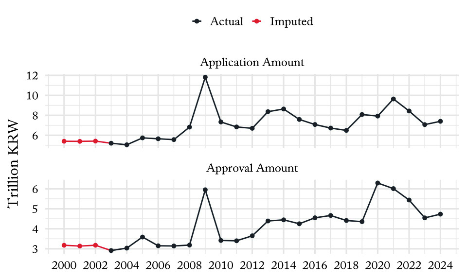
The mean application amount of policy funds is 7.05 trillion KRW and the mean approval amount is 4.12 trillion KRW, with the application amount being 1.71 times the approval amount. The standard deviations of the application amount and approval amount are 1.58 trillion KRW and 1.01 trillion KRW respectively, indicating that the variability of the application amount is greater.
Table 1 presents the descriptive statistics of policy fund variables. The median application amount is 6.83 trillion KRW and the median approval amount is 4.25 trillion KRW. The application amount ranges from 5.05 trillion KRW to 11.81 trillion KRW, and the approval amount ranges from 2.91 trillion KRW to 6.29 trillion KRW.
<Table 1> Descriptive Statistics of Policy Fund Variables
| Variable | Mean | Median | SD | Min | Max |
|---|---|---|---|---|---|
| Application Amount | 7.05 | 6.83 | 1.58 | 5.05 | 11.81 |
| Approval Amount | 4.12 | 4.25 | 1.01 | 2.91 | 6.29 |
* Unit: trillion KRW
Figure 1 presents the time series trend of policy fund variables. The time series fluctuations of policy fund variables show a close association with the business cycle. The approval amount ranges from 2.91 trillion KRW in 2003 to 6.29 trillion KRW in 2020, showing counter-cyclical expansion to 5.95 trillion KRW and 6.29 trillion KRW at the financial crisis of 2009 and the COVID-19 pandemic of 2020, respectively. The application amount also shows a similar pattern, maintaining an average of 1.73 times the approval amount.
4.3 Demand Function Explanatory Variables
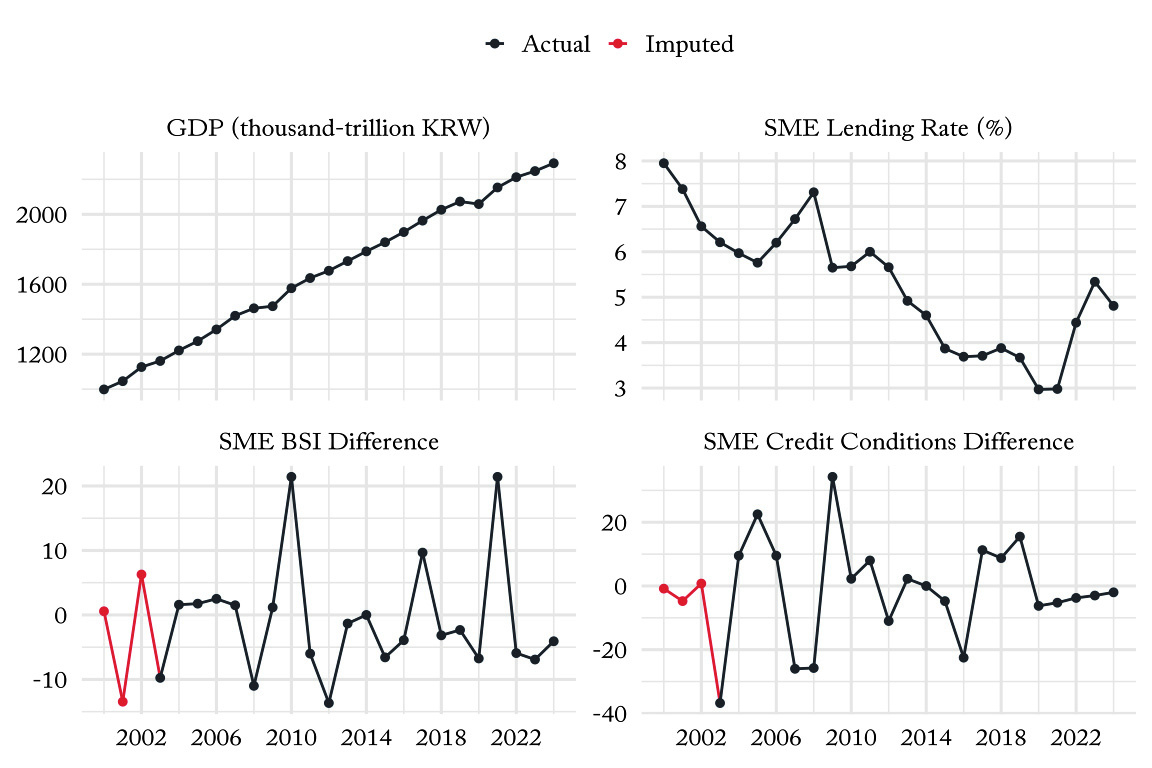
Table 2 presents the descriptive statistics of demand function explanatory variables. GDP continuously grew from 998.29 thousand-trillion KRW in 2000 to 2,292.20 thousand-trillion KRW in 2024. The SME lending rate shows a downward trend from 7.95% in 2000 to 2.97% in 2020. The SME BSI difference fluctuates between -13.67 in 2012 and 21.42 in 2010, 2021, while the SME credit conditions difference fluctuates between -36.75 in 2003 and 34.25 in 2009, reflecting business cycle fluctuations.
<Table 2> Descriptive Statistics of Demand Function Explanatory Variables
| Variable | Mean | Median | SD | Min | Max |
|---|---|---|---|---|---|
| GDP | 1,667.99 | 1,677.09 | 402.53 | 998.29 | 2,292.20 |
| SME Lending Rate | 5.28 | 5.65 | 1.39 | 2.97 | 7.95 |
| SME BSI Difference | -1.08 | -2.33 | 8.85 | -13.67 | 21.42 |
| SME Credit Conditions Difference | -1.12 | -0.83 | 15.55 | -36.75 | 34.25 |
* GDP in thousand-trillion KRW, lending rate in %, others in year-on-year difference
Figure 2 presents the time series trends of demand function explanatory variables. GDP continuously increased throughout the analysis period, while the SME lending rate gradually declined from high levels in the early 2000s, reaching its lowest level in the early 2020s before rising again. The SME BSI difference and credit conditions difference fluctuate with the business cycle, exhibiting particularly large variations at the financial crisis of 2009 and the COVID-19 pandemic of 2020.
4.4 Supply Function Explanatory Variables
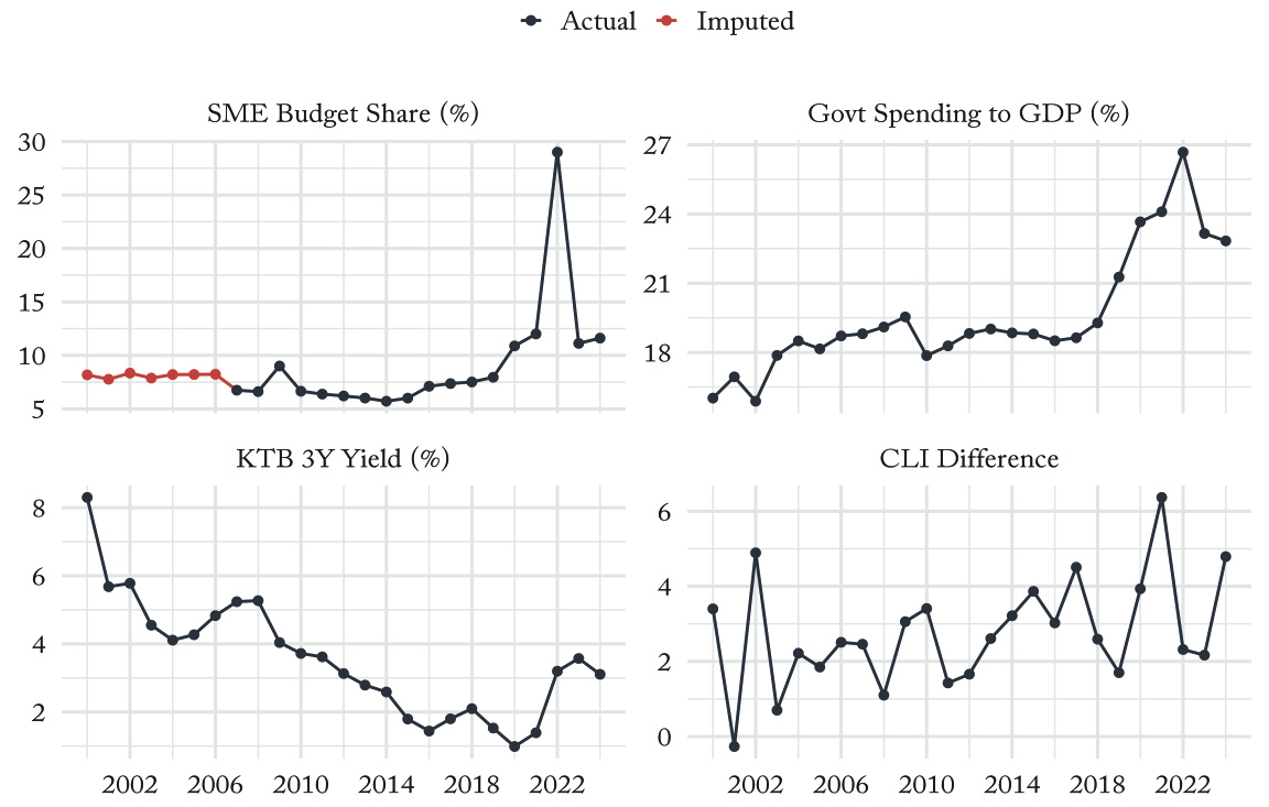
Table 3 presents the descriptive statistics of supply function explanatory variables. The SME budget share was at the normal level of 7.7% but surged to 29.01% in 2022. Government spending to GDP fluctuates between 15.89% in 2002 and 26.68% in 2022, reflecting fiscal expansion during crises. The KTB yield fluctuates between 0.99% in 2020 and 8.30% in 2000, while the CLI difference shows an average of 2.78, indicating that expectations of economic improvement generally prevailed, yet exhibits considerable variability with a standard deviation of 1.45.
<Table 3> Descriptive Statistics of Supply Function Explanatory Variables
| Variable | Mean | Median | SD | Min | Max |
|---|---|---|---|---|---|
| SME Budget Share | 8.83 | 7.88 | 4.56 | 5.71 | 29.01 |
| Govt Spending to GDP | 19.57 | 18.81 | 2.61 | 15.89 | 26.68 |
| KTB 3Y Yield | 3.55 | 3.57 | 1.73 | 0.99 | 8.30 |
| CLI Difference | 2.78 | 2.59 | 1.45 | -0.27 | 6.37 |
* Budget share and government spending in %, KTB yield in %, CLI in year-on-year difference
Figure 3 presents the time series trends of supply function explanatory variables. The SME budget share surged at the COVID-19 pandemic of 2020, and government spending to GDP also shows an expansionary pattern during crisis periods. The KTB yield shows a downward trend from the early 2000s before rising again in the early 2020s. The CLI difference fluctuates reflecting the business cycle.
Ⅴ. Results
5.1 Model Estimation Results
The structure of SME policy fund demand and supply was estimated through the truncated normal distribution model.5) A total of 15 parameters were estimated for 25 observations. To prevent numerical instability arising from scale differences across variables, all explanatory variables were transformed into standardized scores.6)
Table 4 presents the estimation results of the truncated normal distribution model. In the demand function, the GDP coefficient of 0.564 and the lending rate coefficient of -0.398 are statistically significant, confirming that economic growth and interest rate fluctuations are key determinants of policy fund demand. In the supply function, the government spending coefficient of 0.459, the base rate coefficient of -0.341, and the business cycle coefficient of 0.298 are significant, confirming that fiscal policy and monetary policy serve as primary determinants of supply. The application coefficient is estimated at 0.550, suggesting that approximately 55% of the application amount contains pure demand information.
<Table 4> Truncated Normal Distribution Model Estimation Results (Standardized Variables)
| Parameter | Estimate | Parameter | Estimate |
|---|---|---|---|
| Demand Intercept | 0.360* | Base Rate | -0.341* |
| (0.156) | (0.138) | ||
| GDP | 0.564** | CLI | 0.298* |
| (0.160) | (0.097) | ||
| Lending Rate | -0.398** | Supply Variance (sigma_S, log) | -0.685*** |
| (0.103) | (0.142) | ||
| BSI | 0.114 | Application (gamma) | 0.550* |
| (0.066) | (0.186) | ||
| Credit Conditions | 0.089 | Application Variance (sigma_A, log) | -0.209 |
| (0.100) | (0.143) | ||
| Demand Variance (sigma_D, log) | -4.605*** | Excess Demand (delta, log) | -4.605 |
| (0.131) | (4.896) | ||
| Supply Intercept | -0.044 | Num.Obs. | 25 |
| (0.100) | Log.Lik. | -48.644 | |
| Budget Share | 0.014 | AIC | 127.3 |
| (0.063) | BIC | 145.6 | |
| Govt Spending | 0.459* | ||
| (0.169) |
* p<0.05, ** p<0.01, *** p<0.001
5.2 Interpretation of Demand Function Parameters
The GDP coefficient is estimated at 0.564 (p< 0.01), indicating that a one standard deviation increase in standardized GDP is associated with a 0.564 standard deviation increase in policy fund demand, demonstrating a strong positive relationship. This confirms the co-movement of funding demand with SME investment expansion and increased economic activity, and reflects the pro-cyclical demand characteristic in which policy fund demand expands during periods of economic growth.
The SME lending rate coefficient is estimated at -0.398 (p < 0.01), indicating that a one standard deviation increase in the standardized lending rate is associated with a 0.398 standard deviation decrease in policy fund demand. This contradicts the economic intuition that demand for relatively low-cost policy funds should increase when market interest rates rise. This result can be interpreted as follows. When interest rates rise, the overall financial market contracts and policy fund screening standards are also likely to be strengthened, which in turn contracts firms’ fund procurement and decreases policy fund demand. While this result contradicts the typically expected substitutability relationship between policy funds and market funds, it can be interpreted as the overall investment contraction effect from interest rate increases overwhelming the substitution effect. In other words, firms perceive rising interest rates as a signal of economic slowdown and maintain a conservative attitude toward leveraged business expansion. The actual data also exhibits a correlation of -0.844 between policy fund approval amounts and the SME lending rate, consistent with the estimation result.
The SME BSI coefficient is 0.114 and the credit conditions coefficient is 0.089, both showing positive signs but not statistically significant.
5.3 Interpretation of Supply Function Parameters
The government spending coefficient is estimated at 0.459 (p < 0.05), indicating that a one standard deviation increase in standardized government spending to GDP is associated with a 0.459 standard deviation increase in policy fund supply. This reflects the tendency for policy funds to expand during periods of expansionary fiscal stance.
The base rate coefficient is estimated at -0.341 (p < 0.05), indicating that a one standard deviation increase in the standardized KTB yield is associated with a 0.341 standard deviation decrease in policy fund supply. This is interpreted as the government taking a passive stance toward expanding policy funds due to increased borrowing costs. Accordingly, policy fund supply also decreases during monetary policy tightening periods, indicating a synchronization tendency between monetary and fiscal policies.
The CLI coefficient is 0.298 (p < 0.05), indicating that a one standard deviation improvement in the CLI is associated with a 0.298 standard deviation increase in policy fund supply. This reflects the tendency for policy funds to expand when economic prospects improve.
The budget share coefficient is estimated at 0.014 but is not statistically significant.
5.4 Interpretation of Application and Excess Demand Parameters
The application coefficient is estimated at 0.550 (p < 0.05), indicating that approximately 55% of the application amount reflects equilibrium demand. The remaining 45% can be regarded as noise arising from institutional distortions or application practices.7)
The excess demand parameter is estimated at -4.605 (p > 0.05), yielding a very small value of $\delta = e^{-4.605} \approx 0.0100$.8) This implies that the threshold of the truncation condition is located very close to the supply level. A small indicates that the model’s truncation condition is satisfied even when demand only marginally exceeds supply.
5.5 Funding Gap Analysis
The funding gap represents the difference between SMEs’ latent policy fund demand and actual supply, serving as an indicator that quantifies the funding access constraints due to market failure. The magnitude of the funding gap is evaluated by comparing the predicted demand and supply values estimated from the model with the actual approval amounts.
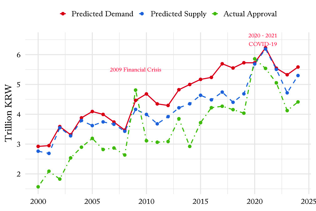
The funding gap analysis, converting the standardized model estimates back to their original scale, yields predicted demand of 2.92 trillion KRW in 2000, continuously increasing to 5.58 trillion KRW in 2024. Predicted supply surged to 5.69 trillion KRW and 6.19 trillion KRW in 2020 and 2021, respectively.
The demand-based average $\lambda$ (the ratio of predicted demand to actual approval) is 1.36, suggesting that latent demand exceeds actual approval by 35.5%. The supply-based average $\lambda$ is 1.24, indicating 24.0% of capacity relative to the actual supply. The appropriate supply of policy funds meets this latent demand, with the appropriate supply quantity corresponding to a $\lambda$-1 multiple expansion of the actual supply. The annual average demand gap over the observation period is 1.07 trillion KRW, indicating that additional supply meeting this gap is required for the appropriate supply of policy funds.
During the economic crises of 2009 and 2020 - 2021, actual approval amounts of 4.81 trillion KRW in 2009, 5.86 trillion KRW in 2020, and 5.54 trillion KRW in 2021 exceeded the predicted values, confirming that policy funds exercised a counter-cyclical function.
Figure 4 presents the time series trend of the funding gap. The predicted demand continuously increased from 2.92 trillion KRW in 2000 to 5.58 trillion KRW in 2024, reflecting structural demand expansion driven by economic growth. The predicted supply maintains a relatively low level compared to demand and surged to 5.69 trillion KRW and 6.19 trillion KRW during the COVID-19 response in 2020 and 2021, confirming crisis-responsive supply expansion. The actual approval remained lower than the predicted supply during normal times but surged to 4.81 trillion KRW during the 2009 financial crisis and to 5.86 trillion KRW and 5.54 trillion KRW during the pandemic of 2020 and 2021, approaching or exceeding the predicted supply level, confirming that the counter-cyclical function of policy funds operated appropriately.
Ⅵ. Conclusion
This study presents a methodology for estimating the appropriate scale of SME policy funds through a structural model in which demand and supply are simultaneously determined. Recognizing that policy fund supply is determined not by a price mechanism but by administrative allocation, the study applies a simultaneous demand-supply determination model to estimate the unobserved latent demand. A truncated normal distribution model employing Bayesian conditional probabilities expresses the structural funding access constraints faced by SMEs with credit ratings of BBB- or below as the equilibrium relationship between demand and supply functions. This approach constitutes an empirical attempt to identify the equilibrium point of demand and supply in the policy financing domain.
The funding gap analysis quantifying the appropriate scale of policy funds shows that latent demand exceeds actual approval by an average of 36%. The equilibrium supply capacity is estimated at 24%, with the annual average demand gap of 1.07 trillion KRW and supply gap of 0.66 trillion KRW over the observation period. During the economic crises of 2009 and 2020 - 2021, actual approval amounts exceeded predicted values, empirically demonstrating the counter-cyclical function of policy funds.
The analysis of the key determinants of demand and supply shows that policy fund demand exhibits a significant positive relationship with GDP growth (coefficient 0.564) and a decreasing pattern with rising SME lending rates (coefficient -0.398). This indicates that policy fund demand is pro-cyclical, and that the investment contraction effect from financial market contraction under rising interest rates overwhelms the substitution effect of policy funds. Policy fund supply increases with expanded government spending to GDP (coefficient 0.459) or improved CLI (coefficient 0.298) and decreases with rising KTB yields (coefficient -0.341), confirming that supply increases with expansionary fiscal stance and improved economic outlook but contracts during monetary tightening. The application coefficient ($\lambda$= 0.550) indicates that approximately 55% of the application amount reflects actual demand, with the remaining 45% interpreted as reflecting strategic overbidding behavior arising from the recognition that only a portion of the application amount will be approved.
6.1 Academic Contribution
This study makes two methodological contributions. First, it demonstrates that a Bayesian structural model based on a truncated normal distribution can be applied to equilibrium analysis of a market without a price mechanism. By decomposing the joint probability of the observed trading volume and the demand constraint into a supply likelihood and a truncation probability, the model identifies latent demand that is not directly observed. Second, the framework that utilizes application and approval data as signals of demand and supply is generalizable to other administratively allocated resources that lack a market price, such as credit guarantees, public housing, and subsidized loans, providing a transferable approach to estimating appropriate supply levels in market failure domains.
6.2 Policy and Practical Implications
The estimated demand gap provides a quantitative reference for budget planning. The annual average demand gap of 1.07 trillion KRW can serve as an empirical basis for setting policy fund budgets in the annual appropriation cycle, replacing incremental adjustments to the previous year’s budget with a gap-based target. The counter-cyclical expansion observed in 2009 and 2020 - 2021 indicates that the timing of supply, not only its scale, matters for crisis response, suggesting that pre-committed expansion rules tied to business cycle indicators can improve the responsiveness of future crisis policy. The application coefficient ($\lambda$ = 0.550) implies that approximately 45% of application amounts reflects strategic overbidding, indicating that mechanisms to curb excessive applications, such as application fees or eligibility pre-screening, can improve allocation efficiency. For SMEs, the gap between latent demand and actual approval informs funding decisions by clarifying the extent of unmet demand, while for financial institutions, the structural excess demand of BBB- and below firms identifies the segment where commercial credit supply is most constrained.
The limitations of this study are as follows. First, the estimation of 15 parameters with 25 observations entails a limitation in statistical estimation efficiency due to the large number of estimation parameters relative to the sample size. Longer data series are expected to reduce the standard errors of estimates and improve numerical stability further. Second, due to the characteristics of the truncated normal distribution model, the likelihood function changes sharply near the truncation point, raising the possibility of numerical instability during optimization. Future research needs to expand the sample size by utilizing quarterly or monthly data and to improve numerical stability and estimation efficiency by introducing alternative estimation methods or regularization techniques.
<Table 5> Funding Gap Analysis Results
| Year | Predicted Demand |
Predicted Supply |
Actual Approval |
Demand Gap |
Supply Gap |
Demand Lambda |
Supply Lambda |
|---|---|---|---|---|---|---|---|
| 2000 | 2.92 | 2.76 | 1.57 | 1.35 | 1.19 | 1.86 | 1.76 |
| 2001 | 2.95 | 2.69 | 2.09 | 0.86 | 0.60 | 1.41 | 1.29 |
| 2002 | 3.59 | 3.55 | 1.83 | 1.76 | 1.72 | 1.96 | 1.94 |
| 2003 | 3.31 | 3.28 | 2.54 | 0.78 | 0.74 | 1.31 | 1.29 |
| 2004 | 3.88 | 3.79 | 2.90 | 0.98 | 0.89 | 1.34 | 1.31 |
| 2005 | 4.09 | 3.62 | 3.19 | 0.90 | 0.43 | 1.28 | 1.13 |
| 2006 | 4.00 | 3.74 | 2.82 | 1.18 | 0.93 | 1.42 | 1.33 |
| 2007 | 3.74 | 3.66 | 2.87 | 0.87 | 0.80 | 1.30 | 1.28 |
| 2008 | 3.47 | 3.43 | 2.63 | 0.83 | 0.80 | 1.32 | 1.30 |
| 2009 | 4.47 | 4.16 | 4.81 | -0.35 | -0.65 | 0.93 | 0.87 |
| 2010 | 4.68 | 4.00 | 3.11 | 1.57 | 0.88 | 1.50 | 1.28 |
| 2011 | 4.35 | 3.68 | 3.06 | 1.29 | 0.62 | 1.42 | 1.20 |
| 2012 | 4.30 | 3.92 | 3.09 | 1.21 | 0.83 | 1.39 | 1.27 |
| 2013 | 4.82 | 4.22 | 3.85 | 0.97 | 0.37 | 1.25 | 1.10 |
| 2014 | 5.00 | 4.35 | 2.92 | 2.08 | 1.43 | 1.71 | 1.49 |
| 2015 | 5.17 | 4.64 | 3.72 | 1.45 | 0.92 | 1.39 | 1.25 |
| 2016 | 5.24 | 4.48 | 4.22 | 1.02 | 0.26 | 1.24 | 1.06 |
| 2017 | 5.69 | 4.74 | 4.27 | 1.42 | 0.47 | 1.33 | 1.11 |
| 2018 | 5.55 | 4.40 | 4.16 | 1.40 | 0.25 | 1.34 | 1.06 |
| 2019 | 5.73 | 4.69 | 4.04 | 1.69 | 0.65 | 1.42 | 1.16 |
| 2020 | 5.73 | 5.69 | 5.86 | -0.13 | -0.17 | 0.98 | 0.97 |
| 2021 | 6.23 | 6.19 | 5.54 | 0.69 | 0.65 | 1.12 | 1.12 |
| 2022 | 5.54 | 5.50 | 5.05 | 0.49 | 0.45 | 1.10 | 1.09 |
| 2023 | 5.33 | 4.72 | 4.12 | 1.20 | 0.60 | 1.29 | 1.14 |
| 2024 | 5.58 | 5.30 | 4.41 | 1.17 | 0.88 | 1.27 | 1.20 |
* Unit: trillion KRW.
Demand Gap = Predicted Demand - Actual Approval.
Supply Gap = Predicted Supply - Actual Approval.
Demand Lambda = Predicted Demand / Actual Approval.
Supply Lambda = Predicted Supply / Actual Approval.